The Pulse of DTX: Expected Patterns, but Questions Remain

Just as people tend to have daily routines, cities follow general patterns throughout the day. Certain areas are crowded during commuting hours, but deserted between morning rush hour and lunchtime. Or perhaps a residential area sees little action until the afternoon when kids come home from school. When combined with the cycles of Earth’s natural systems, these patterns can be explored to reveal the pulse of a city.

Using sensor data collected by the minute from four locations in Boston’s Downtown Crossing (DTX) neighborhood, patterns of atmospheric and environmental conditions illustrate both expected and unexpected information during a hot Thursday in the middle of August.

Summary Information

To begin the investigation, mean values of both air quality and environmental conditions give us a general idea of the type of day DTX had on August 16, 2016.

Variable	Mean	Unit
Humidity	66.39	% RH
Temperature	28.78	Deg C
Luminosity	58.56	Ohms
Sound	68.64	dBA
CO	2.19	voltage
CO2	0.92	voltage
NO2	2.01	voltage
O2	0.56	voltage

Table 1. Mean observation for each variable.

However, these values are averaged over an entire 24 hour period and between two sets of sensors placed in different locations along Washington Street, Winter Street, and Summer Street. A little more digging lets us compare both minimums and maximums of the day as well as relative differences within an approximate 200 foot radius from the intersection of Washington and Winter Streets.

	Humidity		Temperature		Luminosity		Sound
	City 1	City 2	City 1	City 2	City 1	City 2	City 1	City 2
Mean	69.62	63.35	29.25	28.34	70.27	47.56	72.74	64.79
Median	68.75	62.33	28.71	28.39	83.14	54.15	73.00	66.00
Min	47.35	46.56	23.55	23.55	38.42	8.02	64.00	52.00
Max	88.82	77.62	36.77	34.52	97.65	96.19	100.00	95.00

	CO		CO2		NO2		O2
	Environ 1	Environ 2	Environ 1	Environ 2	Environ 1	Environ 2	Environ 1	Environ 2
Mean	1.91	2.41	0.84	0.98	2.01	2.01	0.58	0.54
Median	1.84	2.37	0.82	0.94	2.01	2.00	0.58	0.54
Min	1.34	1.83	0.41	0.75	1.99	1.98	0.55	0.52
Max	3.05	3.30	1.18	1.26	2.08	2.08	0.64	0.61

Table 2. Summary information, separated by sensor location.

Although most of these values are relatively consistent between both sets of sensors, it is interesting to note the difference in luminosity readings between the City 1 and City 2 sensors. City 2 recorded a mean and median luminosity reading significantly below that of City 1 and the minimum reading is an order of magnitude lower.

Luminosity Pattern

But what is causing this difference in luminosity?

luminosity-graph

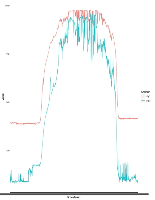
Figure 1. Luminosity readings (Ohms) across 24 hours, by sensor location.

From this graph of luminosity readings recorded across the entire day, the general shape of the data is not too surprising. We would expect lower light levels during the evening hours with a gradual increase and decrease as the sun moves overhead.

Both sensors reach around the same peak in luminosity in the middle of the day. But what is interesting is that the City 1 sensor reaches a steady value overnight which is significantly higher than the irregular readings of the City 2 sensor overnight. This suggests that some areas of DTX remain well lit throughout the night. Perhaps City 1 was located under a street lamp, whereas other areas get quite dark. Additionally, the greater variation in daytime luminosity readings from City 2 indicate this sensor was perhaps in an area subjected to variable shade during the day. What impact would shade have on other recorded conditions?

dtx-1

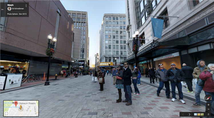
Figure 2. Google Street View of approximate location of City 1 sensor. View looking NW along Summer Street.

Indeed, using Google StreetView, it’s likely that the City 1 sensor was located in close proximity to one entrance of the Downtown Crossing T Station, an area likely to be well lit in the evening.

Sound Pattern

A large contributor to the life and feel of a city is sound. A comparison of sound readings throughout the day from both City 1 and City 2 sensors follows another rather expected pattern.

sound-graph

Figure 3. Sound readings (dBA) across 24 hour period, by sensor location.

For the most part sound levels remain low in the early hours of the morning while people are sleeping. But as the city wakes up, so does the noise, and a gradual increase in sound level is observed, peaking in the late afternoon. A similar pattern to the luminosity readings above is seen here, in which the City 1 sensor remains at a slightly higher, mostly consistent level over night and through parts of the day. Perhaps this is also an expression of the increased activity level surrounding the T station entrance.

However, an unexpected and sharp increase in sound level is captured right around noontime lasting for what must be a few hours*. This pattern is recorded in both sensors, however the City 2 sensor shows a more extreme expression. What happens at this time of day on Winter Street? Was there a street performer with a loudspeaker? Is this simply an expression of the lunchtime rush? Does this happen everyday?

CO and CO2 Patterns

Understanding patterns of air quality throughout the day can both reveal potential sources of pollution as well as indicate areas or times of day when people are most at risk of exposure.

co-graph

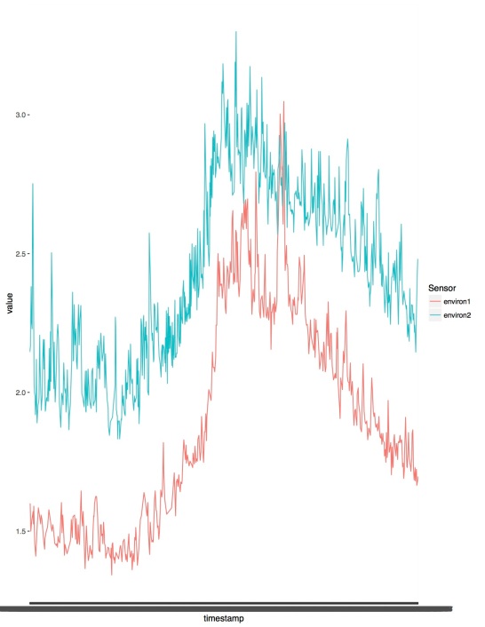
Figure 4. Carbon Monoxide readings (voltage) across 24 hour period, by sensor location.

The daily path of carbon monoxide readings follows an expected pattern. Readings are low in the evening with a gradual increase to a peak during the afternoon. In urban areas, the combustion of fuel in vehicles contribute carbon monoxide into the air. Therefore, it is not surprising that CO levels increase during the day as there are more cars on the road. These sensors are not located on streets with vehicles, however heavily trafficked streets are not far.

It’s interesting, too, that the Environment 2 sensor recorded overall higher readings throughout the entire 24-hour period. Because this relationship is relatively constant throughout the day, it may be factor of calibration between the sensors. Other factors to consider might be nearby construction activities in which heavy machinery or generators could contribute to higher CO concentrations. Or perhaps building or underground parking exhaust from the nearby hotel and high-rise apartments played a role.

dtx2

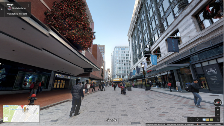
Figure 5. Google Street View of approximate location of Environment 2 sensor. View looking NE along Washington Street.

A final comparison of carbon dioxide readings shows an unusual daily signature. While records remain consistent during the morning hours, a short increase followed by a very sharp decrease is observed around noontime in both sensors.

co2-graph

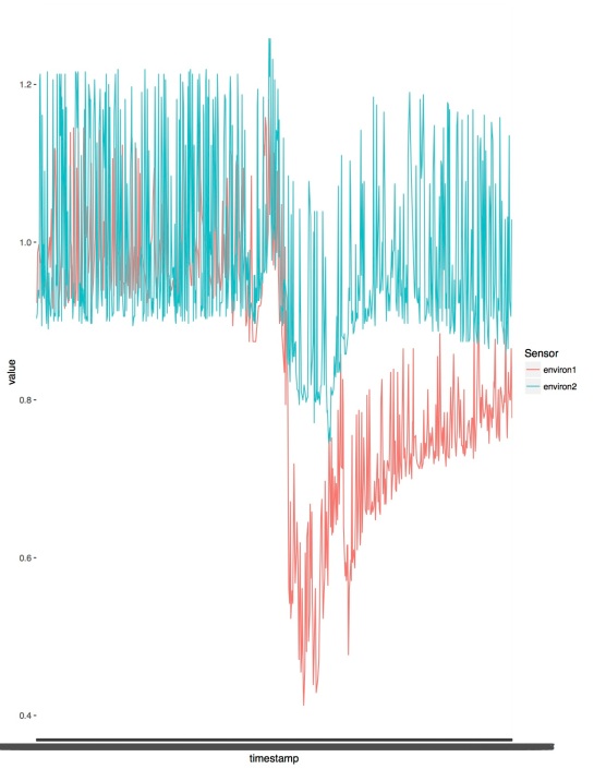
Figure 6. Carbon Dioxide readings (voltage) across 24 hour period, by sensor location.

There are many factors that may contribute to daytime decreases in surface CO2 measurements. For example, as air temperatures increase, convective air mixing can influence concentrations. Or similarly, a change in wind direction may affect readings. But wouldn’t this signature be observed in data from the other air quality variables? And what would have caused such a drastic pattern?

Unusual Patterns and Abnormalities

This dataset has the benefit of only a few variables (ten total), making it relatively small and easy to handle. However, there are a few strange characteristics that may need adjustment in order to fully explore the potential for information.

As mentioned above, there are two particularly strange patterns that emerge when these data are plotted graphically. The first is an unusual sound signature that occurs in the afternoon recorded by the City 2 sensor. What has caused this extreme and sustained spike in decibels? The second is found in the CO2 signature. What could cause relatively consistent readings to drastically drop in a matter of minutes? Is this an actual observation or do the data need to be adjusted?

However, of more interest is the use of units for the sensors’ atmospheric observations. The Environment sensors both capture information regarding concentrations of CO, CO2, NO2 and O2 in the air. But the extent to which these data can be compared between sensors and between regulated standards is unclear. When looking into the provided metadata for this dataset, the units for each of these variables is indicated as “voltage” which can be inferred to represent the direct reading from the electrochemical sensors. However, most information regarding regulated concentrations of air pollutants is given in ppm or ppb. Identifying the relationship between these voltage signals and common concentration units will help turn these observations into more meaningful information.

Furthermore, if the voltage signals are based on a calibration setting unique to each sensor, it may be necessary to determine the relationship between Environment 1 and Environment 2. For example, the carbon monoxide readings had very similar patterns from both sensors but were off by about 0.5 volts. Is this a significant difference between the physical sensor locations or do the data need to be normalized?

One last unusual item regards the number of observations within these datasets. When separated by sensor or by type of record, the number of observations is not consistent. For example, Environment 1 recorded 2,262 observations but Environment 2 recorded 2,897 observations. Similarly, there were 2,328 temperature readings from City 1 but 2,317 humidity readings from the same sensor. After just a brief review of the raw data, there appears to be occasional duplicates. Sensor Environment 1 recorded a CO value of 1.5 at time 00:02:16 twice. These duplicates may slightly skew summary results and will need to be identified and removed.

While many questions remain, these patterns help to form a picture of the daily conditions of DTX in August. It’s interesting to wonder what these patterns look like in different seasons and different parts of the city.

-Ellie

Appendix: Code

‘find mean of each type of value recorded

‘data frames named: sensorA and sensorB

> by(sensorA$value, sensorA$sensor, mean)

sensorA$sensor: GP_HUM

[1] 66.39495

————————————————————————

sensorA$sensor: GP_TC

[1] 28.78003

————————————————————————

sensorA$sensor: LUM

[1] 58.56734

————————————————————————

sensorA$sensor: MCP

[1] 68.64488

> by(sensorB$value, sensorB$sensor, mean)

sensorB$sensor: CO

[1] 2.192188

————————————————————————

sensorB$sensor: CO2

[1] 0.9187409

————————————————————————

sensorB$sensor: NO2

[1] 2.007558

————————————————————————

sensorB$sensor: O2

[1] 0.5596685

‘create new data frames to separate information by sensor

> city1<-sensorA[sensorA$id_wasp == “city1”,]

> city2<-sensorA[sensorA$is_wasp == “city2”,]

> environ1<-sensorB[sensorB$id_wasp == “environ1”,]

> environ2<-sensorB[sensorB$id_wasp == “environ2″,]

‘compare summary of each variable across both sensors (eg. 1&2)

> by(city1$value, city1$sensor, summary)

city1$sensor: GP_HUM