Variable Definition
After aggregating the sensor data on a minute-basis from last week, it is possible to continue to build out the sub-latent variables that contribute to our latent variable of Street Comfort.
For each sub-latent variable, a score was established to indicate how that latent variable contributes to the Street Comfort variable. Eventually, the score of each sub-latent variable can be aggregated to give an overall score of Street Comfort for each minute of record where a higher Street Comfort score is undesirable.
Thermal Comfort
Last week, we created a new variable of heat index to describe how temperature and humidity readings contribute to a person’s thermal comfort. Based on the values of heat index indicated by the National Oceanographic and Atmospheric Administration, it is possible to define an additional variable to indicate whether the heat index at a particular minute is comfortable or not. This ranking of thermal comfort was based on the following values of head index:
| Heat Index Value | Description | Thermal Comfort Score |
| <80 | Comfortable | 0 |
| 80 – 89 | Very Warm | 1 |
| 90 – 104 | Hot | 2 |
| 105 – 129 | Very Hot | 3 |
| >130 | Extremely Hot | 4 |
## thermal comfort: scale 0-4
city_ag$thermcomf1<- ifelse(city_ag$heat_index1 < 80, 0,
ifelse(city_ag$heat_index1 >= 80 & city_ag$heat_index1 < 90, 1,
ifelse(city_ag$heat_index1 >= 90 & city_ag$heat_index1 < 105, 2,
ifelse(city_ag$heat_index1 >= 105 & city_ag$heat_index1 < 130, 3,
ifelse(city_ag$heat_index1 >= 130, 4, 0)))))
city_ag$thermalcomf2<- ifelse(city_ag$heat_index2 < 80, 0,
ifelse(city_ag$heat_index2 >= 80 & city_ag$heat_index2 < 90, 1,
ifelse(city_ag$heat_index2 >= 90 & city_ag$heat_index2 < 105, 2,
ifelse(city_ag$heat_index2 >= 105 & city_ag$heat_index2 < 130, 3,
ifelse(city_ag$heat_index2 >= 130, 4, 0)))))
Sensory Quality
The sensory variable is influenced by both sound and light levels.
For the sound component, a new variable was created to rank the decibel level at each minute based on comfort. Using the following decibel thresholds as described by OSHA, each minute was given a sound score between 0 and 4.
| Decibel Level | Description | Sound Score |
| <60 | Normal Conversation | 0 |
| 61 – 85 | City Traffic | 1 |
| 86 – 100 | Subway Train/Harmful | 2 |
| 100 – 112 | Motorcycle/Extremely Uncomfortable | 3 |
| >112 | Rock Concert/Dangerous | 4 |
## sound component: scale 0-4
city_ag$soundrank1<- ifelse(city_ag$city1_mcp <= 60, 0,
ifelse(city_ag$city1_mcp > 60 & city_ag$city1_mcp < 85, 1,
ifelse(city_ag$city1_mcp >= 85 & city_ag$city1_mcp < 100, 2,
ifelse(city_ag$city1_mcp >= 100 & city_ag$city1_mcp < 112, 3,
ifelse(city_ag$city1_mcp >= 112, 4, 0)))))
city_ag$soundrank2<- ifelse(city_ag$city2_mcp <= 60, 0,
ifelse(city_ag$city2_mcp > 60 & city_ag$city2_mcp < 85, 1,
ifelse(city_ag$city2_mcp >= 85 & city_ag$city2_mcp < 100, 2,
ifelse(city_ag$city2_mcp >= 100 & city_ag$city2_mcp < 112, 3,
ifelse(city_ag$city2_mcp >= 112, 4, 0)))))
The light component was a little less straightforward to define, but simpler to code. Because the luminosity readings are given in Ohms and cannot be translated easily to a more standard unit of light measurement, a particular light threshold was determined based on the time of sunrise.
Street comfort may be influenced by light levels with regard to safety, where a dark street may feel unsafe and therefore uncomfortable. In the absence of streetlights (or other artificial light), light levels are controlled by the sun’s position and therefore, comfortable light levels are reached when the sun has risen in the morning. For this variable, it was assumed that the recorded light level at the time of sunrise (5:48am on August 11, 2016) was equal to the lowest light level that would be considered comfortable. The sunrise light level recorded by sensor City2 was used, as it was determined a few weeks ago that the City1 sensor had influence from streetlights.
As such, luminosity levels above the sunrise light level were considered comfortable and scored a value of 0 whereas levels darker than sunrise were considered less comfortable and scored a value of 1.
| Luminosity (Ohm) | Description | Light Score |
| <22.6 | Darker than sunrise | 1 |
| >22.6 | Lighter than sunrise | 0 |
Note that the City2 sensor also likely had some influence from streetlights or other artificial light. But for the purposes of this variable, that influence is considered to be balanced by the fact that it is perhaps still quite dark at the exact minute of sunrise.
Finally, the sound and light components were combined to give an overall score of sensory quality for each minute.
## light component: scale 0-1
city_ag$lightrank1<- ifelse(city_ag$city1_lum >= 22.6, 0, 1)
city_ag$lightrank2<- ifelse(city_ag$city2_lum >= 22.6, 0, 1)
## sensory quality: combine sound and light components
city_ag$sensory1<- city_ag$soundrank1 + city_ag$lightrank1
Air Quality
Air quality is probably the most challenging sub-latent variable to define due to the unclear units of voltage for each type of reading, which cannot be converted to ppm and therefore cannot be compared with any actual standard or measure of comfort.
For the purpose of this variable, it was assumed that the day of record, August 11, 2016, was a typical day for air quality during which levels of each chemical ranged between comfortable and uncomfortable. In reality, this becomes more a measure of “relative” comfort where the actual difference between what is scored as comfortable and uncomfortable may not actually be significantly different.
This measure was scored using the summary data for each chemical in which recorded values between the 25th and 75th quartiles were considered normal and without influence on comfort. Recorded values that were below the 25th or above the 75th percentiles (depending on the chemical) were considered elevated, and values above or below the max or min records, respectively, were considered extreme and uncomfortable. These values, of course, will not occur in this dataset, but may be useful if this variable is applied to sensor data from a different day or location.
Carbon Monoxide Levels
| Reading (voltage) | Description | Sound Score |
| <1.342 | Lower than min | 0 |
| 1.342 – 1.887 | Below normal | 0 |
| 1.887 – 2.514 | Normal | 0 |
| 2.514 – 3.300 | Above normal | 1 |
| >3.300 | Above max | 2 |
Oxygen Levels
| Reading (voltage) | Description | Sound Score |
| <0.516 | Lower than min | 2 |
| 0.516 – 0.539 | Below normal | 1 |
| 0.539 – 0.581 | Normal | 0 |
| 0.581 – 0.635 | Above normal | 0 |
| >0.635 | Above max | 0 |
Mapping Sensor Data
A map of these variables are not quite as valuable as a different type of dataset given that only four sensors were employed, therefore only four points can occur at one time. In addition, the City and Environment sensors were not placed together, therefore combining the thermal comfort and sensory quality variables with the air quality variable is not valid except when considering the area as a whole (and not comparing sensor locations).
It is, however, extremely valuable to have a spatial understanding of where these variables are located. Thus, the first map includes simply the sensor locations.
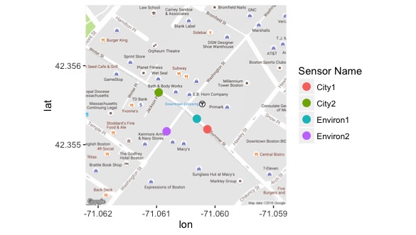
## add sensor locations
sensorname<- c(‘City1’, ‘City2’, ‘Environ1’, ‘Environ2’)
lat<- c(42.355195, 42.355662, 42.355328, 42.355169)
long<- c(-71.060131, -71.060964, -71.060311, -71.060828)
sensor_loc<- data.frame(sensorname, lat, long)
## get basemap
require(rgdal)
require(sp)
require(ggmap)
DTX<- get_map(location=c(left = -71.063, bottom = 42.354, right = -71.058, top = 42.357))
DTXmap<- ggmap(DTX)
DTXmap
base<- DTXmap + geom_point(data=sensor_loc,
aes(x=long, y=lat, color=sensorname), size=3.5) +
scale_color_discrete(name = ‘Sensor Name’)
base
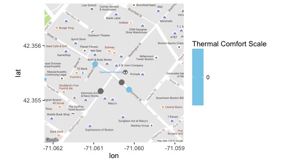
In order to spatial analyze the data at each sensor location, it is necessary to view several maps, each representing a different time of day. For example, the following maps show the thermal comfort level at 6am, 9am, 12pm, 3pm, and 6pm.
6am
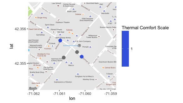
9am
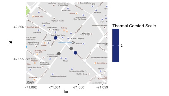
12pm
3pm

## map thermal comfort at particular times
## at 6am
thermal_comfort<- c(city_ag[city_ag$hour == 6 & city_ag$minute == 0, 17],
city_ag[city_ag$hour == 6 & city_ag$minute == 0, 28], NA, NA)
city_map_df<- data.frame(sensorname, lat, long, thermal_comfort)
DTXmap + geom_point(data=city_map_df, aes(x=long, y=lat, color=thermal_comfort), size = 3.5) +
scale_color_continuous(name = “Thermal Comfort Scale”, low = “skyblue”, high = “skyblue”)
## at 9am
thermal_comfort<- c(city_ag[city_ag$hour == 9 & city_ag$minute == 0, 17],
city_ag[city_ag$hour == 9 & city_ag$minute == 0, 28], NA, NA)
city_map_df<- data.frame(sensorname, lat, long, thermal_comfort)
DTXmap + geom_point(data=city_map_df, aes(x=long, y=lat, color=thermal_comfort), size = 3.5) +
scale_color_continuous(name = “Thermal Comfort Scale”, low = “royalblue”, high = “royalblue”)
## at 12pm
thermal_comfort<- c(city_ag[city_ag$hour == 12 & city_ag$minute == 0, 17],
city_ag[city_ag$hour == 12 & city_ag$minute == 0, 28], NA, NA)
city_map_df<- data.frame(sensorname, lat, long, thermal_comfort)
DTXmap + geom_point(data=city_map_df, aes(x=long, y=lat, color=thermal_comfort), size = 3.5) +
scale_color_continuous(name = “Thermal Comfort Scale”, low = “royalblue4”, high = “royalblue4”)
## at 3pm
thermal_comfort<- c(city_ag[city_ag$hour == 15 & city_ag$minute == 0, 17],
city_ag[city_ag$hour == 15 & city_ag$minute == 0, 28], NA, NA)
city_map_df<- data.frame(sensorname, lat, long, thermal_comfort)
DTXmap + geom_point(data=city_map_df, aes(x=long, y=lat, color=thermal_comfort), size = 3.5) +
scale_color_continuous(name = “Thermal Comfort Scale”, low = “royalblue4”, high = “royalblue4”)
## at 6pm
thermal_comfort<- c(city_ag[city_ag$hour == 18 & city_ag$minute == 0, 17],
city_ag[city_ag$hour == 18 & city_ag$minute == 0, 28], NA, NA)
city_map_df<- data.frame(sensorname, lat, long, thermal_comfort)
DTXmap + geom_point(data=city_map_df, aes(x=long, y=lat, color=thermal_comfort), size = 3.5) +
scale_color_continuous(name = “Thermal Comfort Scale”, low = “royalblue4”, high = “royalblue4”)
