- Intro
So far, I have been focusing on local business in Boston. This is interesting because it could reveal some clues about local economy. For example, if a certain area has lots of local business than other areas have, it might be reasonable guess that the area would have higher level of local investment coming from a number of local businesses generate.
I would like to prove this ‘reasonable guess’ by proper analysis tools so decided to conduct correlation and regression between local business and local investment using the two data, business license and census tracts.
- Data Merge
First of all, I needed to merge those two data in the tract-level. While I was trying to merge the tract-level estimates for local investment to business license directly, I noticed that it resulted some problems caused by the merging the two different level. For this reason, I calculated the number of local business by census tracts, CT_ID_10. After that, I merged this aggregated data set which names “avg_local” to the tract-level local investment.
##Define local##
business$local <- ifelse(business $STATE == business$COSTATE,1,0)
##Create new data set, state##
state<-business[business$local==”1″,]
##Calculate the number of local business by census tracts##
avg_local<-aggregate(cbind(local)~state$CT_ID_10,data=state,sum)
names(avg_local)[1]<-‘CT_ID_10′
##Merge avg local to local investment##
tracts<-merge(CT_All_Ecometrics_2014,avg_local,by=’CT_ID_10’,all.x=TRUE)
- Correlation
Before I conducted the correlation between the number of local business and local investment, I expected those two should be positive correlation, which means when the tract has higher number of local business, the level of local investment has to be higher. As a result, the correlation is positive even though the degree is not strong. (cor= 0.02)
##Correlation##
cor(tracts$Local_Investment_2014,tracts$local,use = “complete”)
[1] 0.02043934
However, it was too early to conclude that those two variables have causal relationship because I was not sure that their movement in same direction (positive correlation) also can guarantee the influence of one variable on the other variable. In order to know this, I did regression analysis.
- Regression
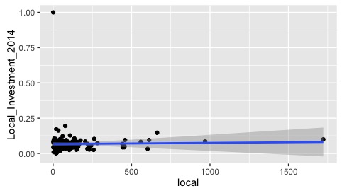
So my research hypothesis was that there is a linear relationship between local and local investment. After the regression, I could not accept the hypothesis because the p value is 0.788 which is greater than 0.05. So I cannot reject the null hypothesis which is there is no linear relationship between local and local investment. I was able to confirm this numeric result with a scatter plot as below.
#Regression between local and local investment##
> install.packages(“QuantPsyc”)
> regression<-lm(local~Local_Investment_2014,data=tracts)
summary(regression)
##Creating pplot##
> require(ggplot2)
> base<-ggplot(data=tracts,aes(x=local,y=Local_Investment_2014))+geom_point()
> base
>base+geom_smooth(method=lm)
