Comparing Groups in Cambridge

This week, I wanted to examine some of my constructs in more detail at the parcel level (I used parcel level as of now due to the larger sample size for quantitative analysis). The data for this week uses the building permit data as well as the year built and total home value for the parcel.

“`{r include=FALSE}
library(readr)
library(dplyr)
library(lubridate)
library(curl)
library(devtools)
library(ggplot2)
library(sqldf)
library(stringr)
library(easyGgplot2)
library(readr)
library(aCRM)
require(rgdal)
require(sp)
require(ggmap)
library(sf)
require(Hmisc)
library(corrplot)
library(data.table)
require(reshape2)
require(ggplot2)
blockc<-read.csv(‘~/Desktop/Big Cities/blockc.csv’)
names(blockc)
“`

First, I want to compare whether parcels that have energy-related permits differ in years built, total value, and total cost of construction.

t.test(total_cost~energy_inv, data=blockc)
t.test(TOTAL_VAL~energy_inv, data=blockc)
t.test(YEAR_BUILT~energy_inv, data=blockc)

t.test(TOTAL_VAL~solar_iv, data=blockc)
t.test(YEAR_BUILT~solar_iv, data=blockc)
t.test(total_cost~solar_iv, data=blockc)

Surprisingly, I found no significant results in terms of group differences between parcels with and without energy-related permits. I also broke this down by types of energy permits to further examine group differences, but also did not find significant differences.

	Welch Two Sample t-test

data:  TOTAL_VAL by solar_iv
t = 1.4409, df = 2370.4, p-value = 0.1498
alternative hypothesis: true difference in means is not equal to 0
95 percent confidence interval:
 -175802.2 1149901.9
sample estimates:
mean in group 0 mean in group 1 
      1372496.7        885446.9 


	Welch Two Sample t-test

data:  YEAR_BUILT by solar_iv
t = 0.66792, df = 275.84, p-value = 0.5047
alternative hypothesis: true difference in means is not equal to 0
95 percent confidence interval:
 -14.42075  29.23118
sample estimates:
mean in group 0 mean in group 1 
       1896.019        1888.614 


	Welch Two Sample t-test

data:  total_cost by solar_iv
t = -1.0054, df = 254.08, p-value = 0.3156
alternative hypothesis: true difference in means is not equal to 0
95 percent confidence interval:
 -1200806.6   389100.2
sample estimates:
mean in group 0 mean in group 1 
       104801.2        510654.4 

Next, I examined whether tracts differ in the number of energy permits and found that they, in fact, do differ in the number of permits.

blockc$TRACTCE10<- as.factor(blockc$TRACTCE10)
anova<-aov(num_perm_energy~TRACTCE10, data=blockc)
class(anova)
summary(anova)

[1] "aov" "lm" 
              Df Sum Sq Mean Sq F value Pr(>F)  
TRACTCE10     32   13.8  0.4303   1.599  0.018 *
Residuals   2541  683.9  0.2691                 
---
Signif. codes:  0 ‘***’ 0.001 ‘**’ 0.01 ‘*’ 0.05 ‘.’ 0.1 ‘ ’ 1
2 observations deleted due to missingness

 

Finally, for the next set of analyses, I looked at the proportion of energy-related permits as a continuous dependent variable to examine certain characteristics in greater detail. For this, I examined whether parcels with a greater proportion of energy permits differ in total cost of construction, split up into categorical groups.

“`{r}
anova<-aov(prop_energy~TC, data=blockc)
class(anova)
summary(anova)
“`

[1] "aov" "lm" 
              Df Sum Sq Mean Sq F value Pr(>F)  
TC             3   0.91  0.3026   2.829 0.0372 *
Residuals   2570 274.91  0.1070                 
---
Signif. codes:  0 ‘***’ 0.001 ‘**’ 0.01 ‘*’ 0.05 ‘.’ 0.1 ‘ ’ 1
2 observations deleted due to missingness

Results find significant differences across the cost of construction.

TukeyHSD(anova)

Tukey multiple comparisons of means
    95% family-wise confidence level

Fit: aov(formula = prop_energy ~ TC, data = blockc)

$TC
                                                  diff
100,000 and 499,999-0 and 99,999          -0.045695618
500,000 and 1MIL-0 and 99,999             -0.040398627
greater than one mill-0 and 99,999        -0.035326424
500,000 and 1MIL-100,000 and 499,999       0.005296991
greater than one mill-100,000 and 499,999  0.010369194
greater than one mill-500,000 and 1MIL     0.005072203
                                                  lwr
100,000 and 499,999-0 and 99,999          -0.08818622
500,000 and 1MIL-0 and 99,999             -0.14060169
greater than one mill-0 and 99,999        -0.18515309
500,000 and 1MIL-100,000 and 499,999      -0.10021323
greater than one mill-100,000 and 499,999 -0.14305761
greater than one mill-500,000 and 1MIL    -0.17318319
                                                   upr
100,000 and 499,999-0 and 99,999          -0.003205019
500,000 and 1MIL-0 and 99,999              0.059804438
greater than one mill-0 and 99,999         0.114500241
500,000 and 1MIL-100,000 and 499,999       0.110807214
greater than one mill-100,000 and 499,999  0.163795993
greater than one mill-500,000 and 1MIL     0.183327598
                                              p adj
100,000 and 499,999-0 and 99,999          0.0292937
500,000 and 1MIL-0 and 99,999             0.7280345
greater than one mill-0 and 99,999        0.9301587
500,000 and 1MIL-100,000 and 499,999      0.9992325
greater than one mill-100,000 and 499,999 0.9981370
greater than one mill-500,000 and 1MIL    0.9998597

I then plotted this using GGPLOT2 in order to visualize the differences between groups.

melted<-melt(blockc[c(11,22)],id.vars=c(“TC”))
means<-aggregate(value~TC,data=melted,mean)
names(means)[2]<-“mean”
ggplot(data=means, aes(x=TC, y=mean)) + geom_bar(stat=”identity”,position=”dodge”, fill=”blue”) + ylab(“Mean”)

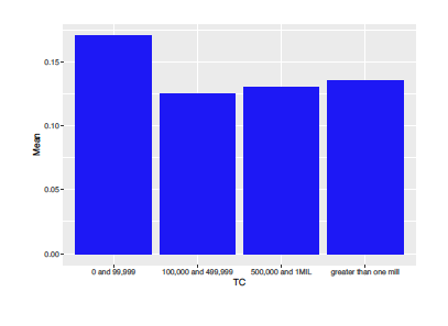
This shows that the proportion of parcels with energy-related permits may be more likely to fall below that 100,000-5000,000 price point but be in fact less expensive. This is an interesting finding!