For my tests, I want to look at different types of zoning, and the effect that might have on the number of landscape-altered parcels. The first part of this post creates a category for zoning, looking at how each parcel in Newton is zoned. The second part of this creates my manifest variable for landscape alteration. Originally, I had been aggregating landscape-altering permits, but comments on my midterm recommended trying looking at the number of parcels that had at least one of the permits, so as not to over-count parcels with several such permits, so this required some tweaked code. Finally, I get to testing the difference. I run a t-test to compare parcels zoned for residential single-family versus multi-family. I will then run an anova analysis looking at the difference in mean variance in the five types of zoning.
Setting things up
require(tidyverse)
library(lubridate)
library(rgdal)
library(maptools)
library(rgeos)
library(maps)
library(ggmap)
library(Hmisc)
library(QuantPsyc)
library(scales)
library(censusapi)

newtonBuilding <- read_csv("nw_BP_clean.csv") # I cleaned the new building permit data in a different file
Here I create my use categories. They are residential for single family, residential for multifamily, business, mixed use, and “other” as a catch-all. For zoning codes, go to http://www.newtonma.gov/gov/it/gis/gis_zoning.asp
newtonTax <- read_csv("Newton_TAcensus.csv")
newtonTax <- newtonTax %>%
  mutate(ResidentMulti = ifelse(grepl("MR",ZONING),"Resident_Multi",NA)) %>%
  mutate(ResidentSingle = ifelse(grepl("SR",ZONING),"Resident_Single",NA)) %>%
  mutate(MultiUse = ifelse(grepl("MU",ZONING),"Mixed",NA)) %>%
  mutate(BusinessUse1 = ifelse(grepl("BU",ZONING),"Business",NA)) %>%
  mutate(BusinessUse2 = ifelse(grepl("LMD",ZONING),"Business",NA)) %>%
  mutate(BusinessUse3 = ifelse(grepl("MAN",ZONING),"Business",NA)) %>%
  mutate(OtherUse1 = ifelse(grepl("ORD",ZONING),"Other",NA)) %>%
  mutate(OtherUse2 = ifelse(grepl("PUB",ZONING),"Other",NA)) %>%
  mutate(Zoning_Use = coalesce(ResidentMulti,ResidentSingle,MultiUse,BusinessUse1,BusinessUse2,BusinessUse3, OtherUse1,OtherUse2)) %>%
  dplyr::select(-c(ResidentMulti,ResidentSingle,MultiUse,BusinessUse1,BusinessUse2,BusinessUse3, OtherUse1,OtherUse2))
Back to setting up parcels with block groups
totalTaxValue <- newtonTax %>%
  group_by(LOC_ID) %>%
  summarise(totalTaxValue=sum(TOTAL_VAL))

geoTaxValue <- newtonTax %>%
  distinct(LOC_ID, .keep_all = TRUE) %>%
  dplyr::select(LOC_ID,ZIP,TRACTCE10,BG_ID,Zoning_Use)
totalTaxValue <- inner_join(totalTaxValue,geoTaxValue)
## Joining, by = "LOC_ID"
Creating my variable. I am still going to get the total number of the permits, and later make a boolean for if the parcel had any of these
allAdditions <- newtonBuilding %>%
  filter(Permit.Type!="BUILD-D" | Permit.Type!="BUILD-N") %>%
  filter(grepl("[Aa]dd+",Note.Text) | Applied.Value > 100000) %>% # this picks up any note with the term add or addition, captialized or not. It also picks up any change over $100,000, which I asusme to be a noticable alteration.
  group_by(LOC_ID, addYear = year(Issue.Date)) %>% #preserving the year information, for trend analysis later
  summarise(addPermit=n(), addPermitValue=sum(Applied.Value))

allNew <- newtonBuilding %>%
  filter(Permit.Type=="BUILD-N") %>%
  group_by(LOC_ID, newYear = year(Issue.Date)) %>% #preserving the year information, for potential trend analysis later
  summarise(newPermit=n(), newPermitValue=sum(Applied.Value))

allDemo <- newtonBuilding %>%
  filter(Permit.Type=="BUILD-D") %>%
  group_by(LOC_ID, demoYear = year(Issue.Date)) %>% #preserving the year information, for potential trend analysis later
  summarise(demoPermit=n(), demoPermitValue=sum(Applied.Value))

allReplace <- merge(allNew,allDemo,by="LOC_ID",all=TRUE) # I combined them here, in case there was value in analyzing just these.

landscapeChangeTotal <- merge(allAdditions, allReplace, by="LOC_ID",all=TRUE) %>%
  group_by(LOC_ID) %>%
  summarise(addPermit=sum(addPermit), addPermitValue=sum(addPermitValue), newPermit=sum(newPermit), newPermitValue=sum(newPermitValue), demoPermit=sum(demoPermit), demoPermitValue=sum(demoPermitValue)) %>%
  mutate(totalPermits = dplyr::select(., c(addPermit,demoPermit,newPermit)) %>% apply(1, sum, na.rm=TRUE)) %>%
  mutate(permitExist = ifelse(totalPermits>0,TRUE,FALSE)) # Creating a true/false if a parcel had a landscape altering variable. This is a recommend change from the midterm
geoLandscape <- merge(totalTaxValue, landscapeChangeTotal, by="LOC_ID",all.x=TRUE)
Analysis
Here, I am creating a table with block groups, the zoning use, the number of altered parcels, the number of total parcels, and the percent altered
landscapeAlterByZoning <- geoLandscape %>%
  group_by(BG_ID,Zoning_Use) %>%
  summarise(landscapeChangingPermittedParcels=sum(permitExist, na.rm=TRUE),totalParcels=n()) %>%
  mutate(percentAltered = landscapeChangingPermittedParcels/totalParcels)
I am particularly interested in the difference in percent altered between multi-family and single-family residential. Before running a t-test, I’ll look at the plot of the two distributions.
laAlterResidential <- landscapeAlterByZoning %>%
  filter(grepl("Resident",Zoning_Use))

laZ <- ggplot(data=laAlterResidential, aes(percentAltered, color=Zoning_Use)) + geom_density() + ggtitle("Distribution of Percent of Landscape Altering Permits by Zoning Type")
laZ
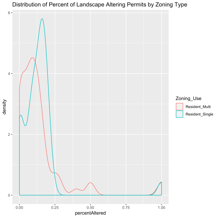
Looking at the graph, the mean looks a little higher for single family, but the multi-family has a slightly longer tail, so the difference is likely not that much. I am going to separate these two uses out explicitly for testing
laResidentSingle <- landscapeAlterByZoning %>%
  filter(Zoning_Use=="Resident_Single") %>%
  dplyr::select(percentAltered)
## Adding missing grouping variables: `BG_ID`
laResidentMulti <- landscapeAlterByZoning %>%
  filter(Zoning_Use=="Resident_Multi") %>%
  dplyr::select(percentAltered)
## Adding missing grouping variables: `BG_ID`
t.test(laResidentSingle$percentAltered,laResidentMulti$percentAltered)
##
##  Welch Two Sample t-test
##
## data:  laResidentSingle$percentAltered and laResidentMulti$percentAltered
## t = 0.23905, df = 122.82, p-value = 0.8115
## alternative hypothesis: true difference in means is not equal to 0
## 95 percent confidence interval:
##  -0.05465220  0.06966539
## sample estimates:
## mean of x mean of y
## 0.1433981 0.1358915
Running the t-test, it does not look like the mean of these varies by much at all. The p-value is so high, it very much looks like the difference could just be from chance, and not from a difference of zoning type.
landscapeAlterByZoning <- landscapeAlterByZoning%>%
  filter(!is.na(BG_ID))

anova <- aov(percentAltered~Zoning_Use, data=landscapeAlterByZoning)
summary(anova)
##              Df Sum Sq Mean Sq F value  Pr(>F)
## Zoning_Use    4  0.467 0.11666   4.415 0.00183 **
## Residuals   245  6.474 0.02643
## ---
## Signif. codes:  0 '***' 0.001 '**' 0.01 '*' 0.05 '.' 0.1 ' ' 1
tukeyTest<- TukeyHSD(anova)
tukeyTest
##   Tukey multiple comparisons of means
##     95% family-wise confidence level
##
## Fit: aov(formula = percentAltered ~ Zoning_Use, data = landscapeAlterByZoning)
##
## $Zoning_Use
##                                       diff          lwr         upr
## Mixed-Business                 -0.10517064 -0.371037368  0.16069609
## Other-Business                 -0.12182792 -0.205308187 -0.03834765
## Resident_Multi-Business        -0.06746543 -0.153354918  0.01842406
## Resident_Single-Business       -0.04384890 -0.128595054  0.04089725
## Other-Mixed                    -0.01665728 -0.279978713  0.24666415
## Resident_Multi-Mixed            0.03770521 -0.226389897  0.30180032
## Resident_Single-Mixed           0.06132174 -0.202403750  0.32504722
## Resident_Multi-Other            0.05436249 -0.023290994  0.13201598
## Resident_Single-Other           0.07797902  0.001592045  0.15436599
## Resident_Single-Resident_Multi  0.02361653 -0.055396252  0.10262930
##                                    p adj
## Mixed-Business                 0.8130811
## Other-Business                 0.0007614
## Resident_Multi-Business        0.1991033
## Resident_Single-Business       0.6141004
## Other-Mixed                    0.9997943
## Resident_Multi-Mixed           0.9949655
## Resident_Single-Mixed          0.9685224
## Resident_Multi-Other           0.3074057
## Resident_Single-Other          0.0428105
## Resident_Single-Resident_Multi 0.9238471
Doing an ANOVA analysis, there is a statistically significant difference in the means of the percent of landscape altering permits by zoning. Doing a Tukey test, it looks like the significant difference is between Other and Business, and Other and Single Resident. Other is the combination of open space zoning and public use zoning. These would both be controlled by the city, and likely the only zoned areas controlled by the city. That the city acts differently than homeowners and businesses in not surprising, but it is something. From the graph above, they do not do much with landscape-altering permits.
